Read custom data in UE4

Posted on February 14, 2021February 14, 2021 by Giorgos Kourakos

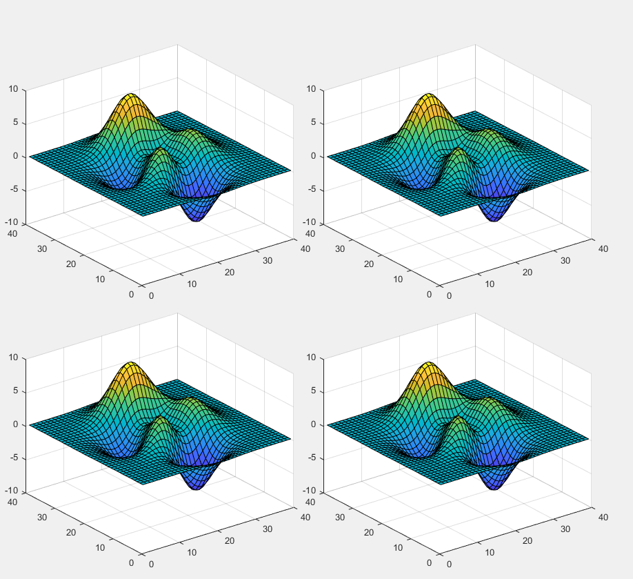
I have recently started looking into ways to use Unreal Engine 4 for my visualizations and so far it looks quite promising. The data I usually work come from groundwater modeling simulations, therefore are not typical data one gets from modeling software such as Blender Houdini etc.

So the following is my way to get data from custom ascii files to UE4. For this guide I will assume that the data are organized as follows:

Nnodes Ntriangles
X Y Z1 Z2 Z3
.
.
.
ID1 ID2 ID3
.
.
.

Nnodes Ntriangles

X Y Z1 Z2 Z3

ID1 ID2 ID3

The first line is the number of nodes and the number of triangles. The procedure I’m following accepts only triangular data. so I have actually converted the quadrilaterals to triangles when I created the above file. Then Nnodes times is repeated the line that holds the x y coordinates. Note that in the file I provide 3 z coordinates. These correspond to ground surface, water table and bottom of the aquifer. in my case. Then I’m listing the ids of each of the Ntriangles of the mesh.

Inside UE4 I started from a C++ project and created an class named CustomMesh based on Actor class. The header file is the following

Header file

#pragma once

#include "CoreMinimal.h"
#include "GameFramework/Actor.h"
#include "ProceduralMeshComponent.h"
#include "CustomMesh.generated.h"

UCLASS()
class BUILING_ESCAPE_API ACustomMesh : public AActor
{
	GENERATED_BODY()
	
public:	
	// Sets default values for this actor's properties
	ACustomMesh();

protected:
	// Called when the game starts or when spawned
	virtual void BeginPlay() override;

	virtual void OnConstruction(const FTransform& Transform) override;

public:	
	// Called every frame
	virtual void Tick(float DeltaTime) override;
	UPROPERTY(VisibleAnywhere, BlueprintReadWrite)
	UProceduralMeshComponent* PM;

	UPROPERTY(EditAnywhere, Category= "DATA")
	FString InputFile;
	
	UPROPERTY(EditAnywhere, Category= "DATA")
	float XYScale = 1000.f;

	UPROPERTY(EditAnywhere, Category= "DATA")
	float ZScale = 10.f;
};

#pragma once

#include "CoreMinimal.h"

#include "GameFramework/Actor.h"

#include "ProceduralMeshComponent.h"

#include "CustomMesh.generated.h"

UCLASS()

class BUILING_ESCAPE_API ACustomMesh : public AActor

{

GENERATED_BODY()

public:

// Sets default values for this actor's properties

ACustomMesh();

protected:

// Called when the game starts or when spawned

virtual void BeginPlay() override;

virtual void OnConstruction(const FTransform& Transform) override;

public:

// Called every frame

virtual void Tick(float DeltaTime) override;

UPROPERTY(VisibleAnywhere, BlueprintReadWrite)

UProceduralMeshComponent* PM;

UPROPERTY(EditAnywhere, Category= "DATA")

FString InputFile;

UPROPERTY(EditAnywhere, Category= "DATA")

float XYScale = 1000.f;

UPROPERTY(EditAnywhere, Category= "DATA")

float ZScale = 10.f;

};

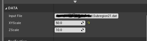
The most important line in the header file is the OnConstruction virtual method which is called every time the asset is transformed. Apart from the virtual method I defined 3 exposed properties InputFile, XYscale, Zscale. There is also a UProceduralMeshComponent that holds the actual data. This actually should not be exposed however I did it as I’m still experimenting with this. This header file will create a category DATA as shown below where the data can be updated inside the editor.

Implementation file
- Constructor

#include "CustomMesh.h"
#include "Misc/FileHelper.h"

// Sets default values
ACustomMesh::ACustomMesh()
{
 	// Set this actor to call Tick() every frame.  You can turn this off to improve performance if you don't need it.
	PrimaryActorTick.bCanEverTick = true;
	
	PM = CreateDefaultSubobject<UProceduralMeshComponent>(TEXT("Procedural mesh"));
	SetRootComponent(PM);
	PM->bUseAsyncCooking = true;

}

#include "CustomMesh.h"

#include "Misc/FileHelper.h"

// Sets default values

ACustomMesh::ACustomMesh()

{

// Set this actor to call Tick() every frame. You can turn this off to improve performance if you don't need it.

PrimaryActorTick.bCanEverTick = true;

PM = CreateDefaultSubobject<UProceduralMeshComponent>(TEXT("Procedural mesh"));

SetRootComponent(PM);

PM->bUseAsyncCooking = true;

}

In the constructor all I’m doing is to create the object and set it as root. Note also that I have included the Filehepler.h which is used for reading the custom file.

- OnConstruction

First we clear out and existing mesh in the object and initialize required variables.

PM->ClearAllMeshSections();
TArray<FString> FileContent;
FVector LowerCorner(999999999.f,999999999.f,999999999.f);
FVector UpperCorner(-999999999.f,-999999999.f,-999999999.f);
FVector Center(0.f, 0.f,0.f);
int Nverts = 0;
int Ntris = 0;
int iline = 0;

FVector T = Transform.GetLocation();

TArray<FVector> GSEVertices;
TArray<FVector> BOTVertices;
TArray<FVector> WTVertices;
TArray<FVector> Normals;
TArray<int32> Indices;
TArray<FColor> ColorVert;

PM->ClearAllMeshSections();

TArray<FString> FileContent;

FVector LowerCorner(999999999.f,999999999.f,999999999.f);

FVector UpperCorner(-999999999.f,-999999999.f,-999999999.f);

FVector Center(0.f, 0.f,0.f);

int Nverts = 0;

int Ntris = 0;

int iline = 0;

FVector T = Transform.GetLocation();

TArray<FVector> GSEVertices;

TArray<FVector> BOTVertices;

TArray<FVector> WTVertices;

TArray<FVector> Normals;

TArray<int32> Indices;

TArray<FColor> ColorVert;

Then I read the first line to get the number of vertices and number of triangles.

const bool bTF = FFileHelper::LoadANSITextFileToStrings(*InputFile,NULL, FileContent);
if (bTF){
    if (FileContent.Num() > 0){
	//Read the number of vertices and triangles
	TArray<FString> Out;
	FileContent[iline].ParseIntoArray(Out, TEXT(" "), true);
	iline++;
	if (Out.Num() > 1){
	    Nverts = FCString::Atoi(*Out[0]);
	    Ntris = FCString::Atoi(*Out[1]);
	}
     }

const bool bTF = FFileHelper::LoadANSITextFileToStrings(*InputFile,NULL, FileContent);

if (bTF){

if (FileContent.Num() > 0){

//Read the number of vertices and triangles

TArray<FString> Out;

FileContent[iline].ParseIntoArray(Out, TEXT(" "), true);

iline++;

if (Out.Num() > 1){

Nverts = FCString::Atoi(*Out[0]);

Ntris = FCString::Atoi(*Out[1]);

}

Next we read the vertices. Note that while reading the x y coordinates we identify the bounding box of the data so that we can translate the mesh into the center of the transform. Otherwise the mesh will be located somewhere far away of the gizmo icon.

if (FileContent.Num() > Nverts)
{
    for (int i = 0; i < Nverts; ++i)
    {
	TArray<FString> Out;
	FileContent[iline].ParseIntoArray(Out, TEXT(" "), true);
	iline++;
	if (Out.Num() > 4)
	{
   	    float x = FCString::Atof(*Out[0])/XYScale + T.X;
	    float y = FCString::Atof(*Out[1])/XYScale + T.Y;
	    float t = FCString::Atof(*Out[2])/ZScale + T.Z;
	    float w = FCString::Atof(*Out[3])/ZScale + T.Z;
	    float b = FCString::Atof(*Out[4])/ZScale + T.Z;
	    if (x > UpperCorner.X) UpperCorner.X = x;
	    if (y > UpperCorner.Y) UpperCorner.Y = y;
	    if (t > UpperCorner.Z) UpperCorner.Z = t;
	    if (x < LowerCorner.X) LowerCorner.X = x;
	    if (y < LowerCorner.Y) LowerCorner.Y = y;
	    if (t < LowerCorner.Z) LowerCorner.Z = t;
	    GSEVertices.Add(FVector(x,y,t));
	    Normals.Add(FVector::UpVector);
	    BOTVertices.Add(FVector(x,y,b));
	    WTVertices.Add(FVector(x,y,w));
	    ColorVert.Add(FColor::MakeRandomColor());
	}
    }
    Center = (UpperCorner + LowerCorner)/2;
    for (int i = 0; i < GSEVertices.Num(); ++i)
    {
	GSEVertices[i] = GSEVertices[i] - Center;
	BOTVertices[i] = BOTVertices[i] - Center;
	WTVertices[i] = WTVertices[i] - Center;
    }
}

if (FileContent.Num() > Nverts)

{

for (int i = 0; i < Nverts; ++i)

{

TArray<FString> Out;

FileContent[iline].ParseIntoArray(Out, TEXT(" "), true);

iline++;

if (Out.Num() > 4)

{

float x = FCString::Atof(*Out[0])/XYScale + T.X;

float y = FCString::Atof(*Out[1])/XYScale + T.Y;

float t = FCString::Atof(*Out[2])/ZScale + T.Z;

float w = FCString::Atof(*Out[3])/ZScale + T.Z;

float b = FCString::Atof(*Out[4])/ZScale + T.Z;

if (x > UpperCorner.X) UpperCorner.X = x;

if (y > UpperCorner.Y) UpperCorner.Y = y;

if (t > UpperCorner.Z) UpperCorner.Z = t;

if (x < LowerCorner.X) LowerCorner.X = x;

if (y < LowerCorner.Y) LowerCorner.Y = y;

if (t < LowerCorner.Z) LowerCorner.Z = t;

GSEVertices.Add(FVector(x,y,t));

Normals.Add(FVector::UpVector);

BOTVertices.Add(FVector(x,y,b));

WTVertices.Add(FVector(x,y,w));

ColorVert.Add(FColor::MakeRandomColor());

}

Center = (UpperCorner + LowerCorner)/2;

for (int i = 0; i < GSEVertices.Num(); ++i)

{

GSEVertices[i] = GSEVertices[i] - Center;

BOTVertices[i] = BOTVertices[i] - Center;

WTVertices[i] = WTVertices[i] - Center;

}

Next we read the triangles. The triangles are stored as 1D vector.

if (FileContent.Num() > Nverts + Ntris)
{
    for (int i = 0; i < Ntris; ++i)
    {
	//UE_LOG(LogTemp, Warning, TEXT("%d"), i);
	TArray<FString> Out;
	FileContent[iline].ParseIntoArray(Out, TEXT(" "), true);
	iline++;
	if (Out.Num() > 2)
	{
	    Indices.Add(FCString::Atoi(*Out[0])-1);
	    Indices.Add(FCString::Atoi(*Out[2])-1);
	    Indices.Add(FCString::Atoi(*Out[1])-1);
	}
    }
}

if (FileContent.Num() > Nverts + Ntris)

{

for (int i = 0; i < Ntris; ++i)

{

//UE_LOG(LogTemp, Warning, TEXT("%d"), i);

TArray<FString> Out;

FileContent[iline].ParseIntoArray(Out, TEXT(" "), true);

iline++;

if (Out.Num() > 2)

{

Indices.Add(FCString::Atoi(*Out[0])-1);

Indices.Add(FCString::Atoi(*Out[2])-1);

Indices.Add(FCString::Atoi(*Out[1])-1);

}

Last we create the custom meshes. For each Z coordinate I create one mesh, which set to visible after the creation.

PM->CreateMeshSection_LinearColor(0, GSEVertices, Indices, TArray<FVector>(), TArray<FVector2D>(), TArray<FLinearColor>(), TArray<FProcMeshTangent>(),true);
PM->CreateMeshSection_LinearColor(1, WTVertices, Indices, TArray<FVector>(), TArray<FVector2D>(), TArray<FLinearColor>(), TArray<FProcMeshTangent>(),true);
PM->CreateMeshSection_LinearColor(2, BOTVertices, Indices, TArray<FVector>(), TArray<FVector2D>(), TArray<FLinearColor>(), TArray<FProcMeshTangent>(),true);
	
/*PM->CreateMeshSection(0, Vertices, Indices,
	Normals,
	TArray<FVector2D>(),
	ColorVert,
	TArray<FProcMeshTangent>(),
	true);*/
PM->SetMeshSectionVisible(0,true);
PM->SetMeshSectionVisible(1,true);
PM->SetMeshSectionVisible(2,true);

PM->CreateMeshSection_LinearColor(0, GSEVertices, Indices, TArray<FVector>(), TArray<FVector2D>(), TArray<FLinearColor>(), TArray<FProcMeshTangent>(),true);

PM->CreateMeshSection_LinearColor(1, WTVertices, Indices, TArray<FVector>(), TArray<FVector2D>(), TArray<FLinearColor>(), TArray<FProcMeshTangent>(),true);

PM->CreateMeshSection_LinearColor(2, BOTVertices, Indices, TArray<FVector>(), TArray<FVector2D>(), TArray<FLinearColor>(), TArray<FProcMeshTangent>(),true);

/*PM->CreateMeshSection(0, Vertices, Indices,

Normals,

TArray<FVector2D>(),

ColorVert,

TArray<FProcMeshTangent>(),

true);*/

PM->SetMeshSectionVisible(0,true);

PM->SetMeshSectionVisible(1,true);

PM->SetMeshSectionVisible(2,true);

So far this is adequate to create the custom mesh. However created a blueprint class based on the Custom Mesh class which I dragged into my scene.

The above code does not read the UV coordinates. Soon I’ll add this info in the file and show some figures.

To be continued…

Subplots in Matlab

Posted on January 20, 2021 by Giorgos Kourakos

One very annoying thing in Matlab subplots is the large space around each subplot.
So the following is a way to overcome this.

To be fair, the credits for the solution goes to … (have a look at this link)

In short the following code, which has been copied from the link above, produces very nice and tight subplots

clf
nRows = 2 ;
nCols = 2 ;
figure() ;
set( gcf, 'Units', 'normalized', 'Position', [0.1, 0.1, 0.5, 0.8] ) ;
[blx, bly] = meshgrid( 0.05:0.9/nCols:0.9, 0.05:0.9/nRows:0.9 ) ;
hAxes = arrayfun( @(x,y) axes( 'Position', [x, y, 0.9*0.9/nCols, 0.9*0.9/nRows] ), blx, bly, 'UniformOutput', false ) ;
for k = 1 : numel( hAxes )
    axes( hAxes{k} ) ;
    surf(peaks(40));
    set( gca, 'Visible', 'on' ) ;
end

clf

nRows = 2 ;

nCols = 2 ;

figure() ;

set( gcf, 'Units', 'normalized', 'Position', [0.1, 0.1, 0.5, 0.8] ) ;

[blx, bly] = meshgrid( 0.05:0.9/nCols:0.9, 0.05:0.9/nRows:0.9 ) ;

hAxes = arrayfun( @(x,y) axes( 'Position', [x, y, 0.9*0.9/nCols, 0.9*0.9/nRows] ), blx, bly, 'UniformOutput', false ) ;

for k = 1 : numel( hAxes )

axes( hAxes{k} ) ;

surf(peaks(40));

set( gca, 'Visible', 'on' ) ;

end

GIS projections in Matlab and R

Posted on December 2, 2020December 2, 2020 by Giorgos Kourakos

In spatial analysis it is very common to gather GIS layers from a variety of sources and more than often the layers may have different coordinate systems. Every GIS software know how to project each layer that comes with different projection information (The projection information is saved in a separate file with suffix *.prj) and can perform spatial analysis tasks on layers with different projection system.

In Matlab and R however the spatial analysis operations work only if the layers have the same coordinate system. Luckily both languages provide functions to convert between projections. Matlab introduced some functions that help with the transformation in the latest update 2020b. So the following will not work in any previous Matlab version not even in 2020a.

Matlab

First let’s bring a couple of data into Matlab workspace. The first layer is a point layer with well locations and the second layer contains the Subregions of the C2Vsim model groundwater basins. For the first layer the *.prj file is missing therefore the coordinate is unknown. For the second file we know from the report that the coordinate system is the EPSG:26910 – NAD83 / UTM zone 10N – Projected.
Mode info about EPSG see here

% For the well layer
% Read the shapefile information
wells_info = shapeinfo('CVwelldata');
% Read the shapefile geometry
wells = shaperead('CVwelldata');

% For the Subregion layer
% Read the shapefile information
C2Vsim_basins_info = shapeinfo('C2Vsim_subBasins');
% Read the shapefile geometry
C2Vsim_basins = shaperead('C2Vsim_subBasins');

% For the well layer

% Read the shapefile information

wells_info = shapeinfo('CVwelldata');

% Read the shapefile geometry

wells = shaperead('CVwelldata');

% For the Subregion layer

% Read the shapefile information

C2Vsim_basins_info = shapeinfo('C2Vsim_subBasins');

% Read the shapefile geometry

C2Vsim_basins = shaperead('C2Vsim_subBasins');

The wells_info.CoordinateReferenceSystem returns an empty field because the projection information is missing. On the other hand C2Vsim_basins_info.CoordinateReferenceSystem returns the following structure

ans = 

  projcrs with properties:

                    Name: "NAD83 / UTM zone 10N"
           GeographicCRS: [1×1 geocrs]
        ProjectionMethod: "Transverse Mercator"
              LengthUnit: "meter"
    ProjectionParameters: [1×1 map.crs.ProjectionParameters]

ans =

projcrs with properties:

Name: "NAD83 / UTM zone 10N"

GeographicCRS: [1×1 geocrs]

ProjectionMethod: "Transverse Mercator"

LengthUnit: "meter"

ProjectionParameters: [1×1 map.crs.ProjectionParameters]

Unfortunately I’m not aware of any automated process to identify the projection system but we can make guesses by examining the coordinate values. If we plot the well data set we get the following image

plot([wells.X]', [wells.Y]','.')
axis equal

1 2	plot([wells.X]', [wells.Y]','.') axis equal

We can see that the range of X and Y coordinates is between -124 – -114 and 33 – 42. If you work with California data this range corresponds to the WGS 84 system with EPSG:4326. This is the coordinate system that many web applications use such as google maps, earth engine etc. use. We can easily verify our assumptions in matlab using the webmap tool. If the coordinate system is indeed 4326 then they should be projected in the right place.

webmap % starts the webmap
wmmarker([wells.Y]', [wells.X]','Alpha',1, 'Color','green', 'IconScale', 0.2, ...
  'Icon','http://maps.google.com/mapfiles/kml/shapes/shaded_dot.png');

webmap % starts the webmap

wmmarker([wells.Y]', [wells.X]','Alpha',1, 'Color','green', 'IconScale', 0.2, ...

'Icon','http://maps.google.com/mapfiles/kml/shapes/shaded_dot.png');

We can see that the well locations fall in the right place. Now we can transform this to any coordinate system using. Note that you may have to switch X and Y

[Wx,Wy] = projfwd(projcrs(3310),[wells.Y]', [wells.X]');

1	[Wx,Wy] = projfwd(projcrs(3310),[wells.Y]', [wells.X]');

Next we have to convert the basin coordinates from EPSG:26910 to EPSG:3310. I haven’t found yet and way to do this transformation using one line so I first convert from EPSG:26910 to EPSG:4326 using projinv and then convert to EPSG:3310. Also because the projinv and projfwd accept only X,Y coordinates not structures we have to loop through the polygons

for ii = 1:length(C2Vsim_basins)
    [lat,lon] = projinv(projcrs(26910),C2Vsim_basins(ii,1).X, C2Vsim_basins(ii,1).Y);
    [C2Vsim_basins(ii,1).X3310, C2Vsim_basins(ii,1).Y3310] = projfwd(projcrs(3310),lat, lon);
end

for ii = 1:length(C2Vsim_basins)

[lat,lon] = projinv(projcrs(26910),C2Vsim_basins(ii,1).X, C2Vsim_basins(ii,1).Y);

[C2Vsim_basins(ii,1).X3310, C2Vsim_basins(ii,1).Y3310] = projfwd(projcrs(3310),lat, lon);

end

Now that the two layers have their coordinates on the same system we can overlay them

plot(Wx,Wy,'.')
hold on
for ii = 1:length(C2Vsim_basins)
    plot(C2Vsim_basins(ii,1).X3310, C2Vsim_basins(ii,1).Y3310,'r')
end

plot(Wx,Wy,'.')

hold on

for ii = 1:length(C2Vsim_basins)

plot(C2Vsim_basins(ii,1).X3310, C2Vsim_basins(ii,1).Y3310,'r')

end

Now that the data sets share the same coordinate system we can do spatial operations. For example we can isolate the wells that are located in the southern most sub-basin of the Central Valley.

in = inpolygon(Wx, Wy, C2Vsim_basins(21,1).X3310, C2Vsim_basins(21,1).Y3310);
plot(Wx(in), Wy(in),'.')
hold on
plot(C2Vsim_basins(21,1).X3310, C2Vsim_basins(21,1).Y3310,'r')

in = inpolygon(Wx, Wy, C2Vsim_basins(21,1).X3310, C2Vsim_basins(21,1).Y3310);

plot(Wx(in), Wy(in),'.')

hold on

plot(C2Vsim_basins(21,1).X3310, C2Vsim_basins(21,1).Y3310,'r')

R

In R the spatial transformations are even easier. First load the library library("rgdal")

The transformation between coordinate system is just one line of code

# Read the data sets
wells &lt;- readOGR(dsn = '.', layer = 'CVwelldata')
C2Vsim_basins &lt;- readOGR(dsn = '.', layer = 'C2Vsim_subBasins')

# Change the coordinate system to 3310
C2Vsim_basins_3310 &lt;- spTransform(C2Vsim_basins, CRS("+init=epsg:3310"))
# Because the wells have no coordinate information first we have to assign the correct one
# we know that this is the 4326
crs(wells) &lt;- CRS('+init=EPSG:4326')
# Now we can make the transformation
wells_3310 &lt;- spTransform(wells, CRS("+init=epsg:3310"))

# Read the data sets

wells <- readOGR(dsn = '.', layer = 'CVwelldata')

C2Vsim_basins <- readOGR(dsn = '.', layer = 'C2Vsim_subBasins')

# Change the coordinate system to 3310

C2Vsim_basins_3310 <- spTransform(C2Vsim_basins, CRS("+init=epsg:3310"))

# Because the wells have no coordinate information first we have to assign the correct one

# we know that this is the 4326

crs(wells) <- CRS('+init=EPSG:4326')

# Now we can make the transformation

wells_3310 <- spTransform(wells, CRS("+init=epsg:3310"))

Subsurface

George Kourakos

Software Tips

Read custom data in UE4

Subplots in Matlab

GIS projections in Matlab and R

Matlab

R