In this post I’ll describe how one can do a simple particle tracking visualization in Houdini.
In general the velocity field will be given, as a product of a simulation for example. For this post we will create a random one
Generate random velocity field
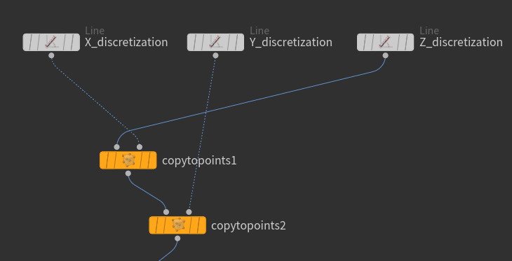
First we create a geometry node and delete the default file node. Then we lay down three line nodes that were renamed as X,Y,Z discretization with the following properties:
Length:1, Points:5 (for start) and Direction {1,0,0}, {0,1,0}, {0,0,1} for the X,Y,Z line respectively.
Then copy the Z line to the points of X and then copy the result to the points of Y. So far we have a 3D grid of points.
Now we are going to assign random velocities on the nodes. Lay down an attribute wrangle node and copy the following code:
|
|
v@v = rand(@ptnum); float w = fit(rand(@ptnum), 0, 1, 0.2, 0.8); v@v = v@v*w; |
The
v@v is read as “declare a vector with name v equal to”.The wrangle node is set to run over points and the
@ptnum is the point id which is used a seed to the rand function that generates a random.
The second line generates a random float value which is scaled between 0.2 and 0.8. Last the velocity vector is scaled using the w value.
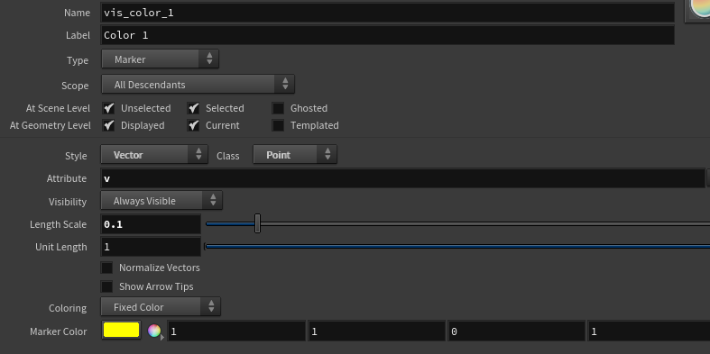
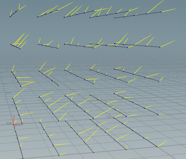
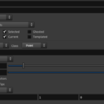
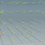
We can visualize the velocity field using the visualize node. Connect the output of the attribute wrangle node to a new visualize node and change under the visualizers tab the type from color to marker the style to vector and choose v as attribute value. You may need to scale the vectors down a bit. (Note also that sometimes you need to go one level up to see the velocity field):
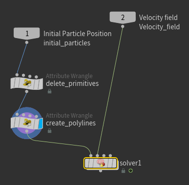
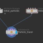
Last select all the nodes that are used for the random velocity field generation and create a subnet (shift+C) and rename it to Velocity field for example.
Generate Random initial particles
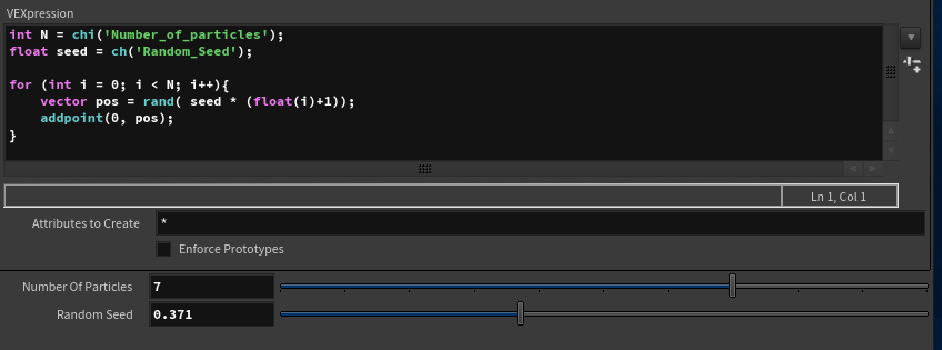
This is another process which most of the time is not random as the initial particle positions are defined by the problems. However here we will generate random initial particles within the space 0 1. This involves just on attribute wrangle node with the following code
|
|
int N = chi('Number_of_particles'); float seed = ch('Random_Seed'); for (int i = 0; i < N; i++){ vector pos = rand( seed * (float(i)+1)); addpoint(0, pos); } |
The first two lines generate GUI elements for this node. After inserting these two lines press the highlighted button which looks like sliders. This will generate two sliders below the code area.
With these two sliders we are able to change the number of particles and the random seed without writing code.
Velocity interpolation
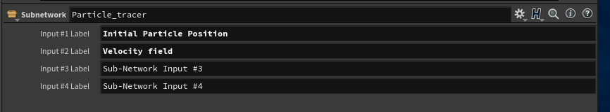
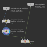
Now its time to write the code for the velocity interpolation. Just to stay organized lay down a null node (which is doing absolutely nothing) and with the null node selected press Shift+C to create a subnet and rename the subnet as Particle tracer. Change also the input labels as follows:
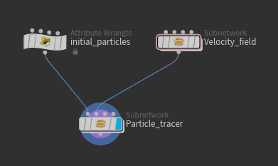
and the network so far looks like the following:
Double click to enter the Particle tracer node and delete the null node.
The first input is expected to be a number of points with the initial particle positions. It is possible that these points form primitives which we don’t want. therefore we will make sure that the primitives are deleted. Lay down an attribute wrangle node, rename it to delete primitives and set its Run Over option to Primitives. There is only one line of code for this wrangle node:
|
|
removeprim(0, @primnum, 0); |
Now that we are sure that there are no primitives, we will create one primitive per particle, a polyline of the trajectory of the particle within the velocity field. Add another attribute wrangle node, rename it to create polylines and leave the Run Over option to Points. Paste the following two lines which, for each point add a primitive and vertex. At this point the primitives cannot be displayed. we need at least two vertices to display a line.
|
|
int iprim = addprim(0, "polyline"); addvertex(0, iprim, @ptnum); |
Setup solver node
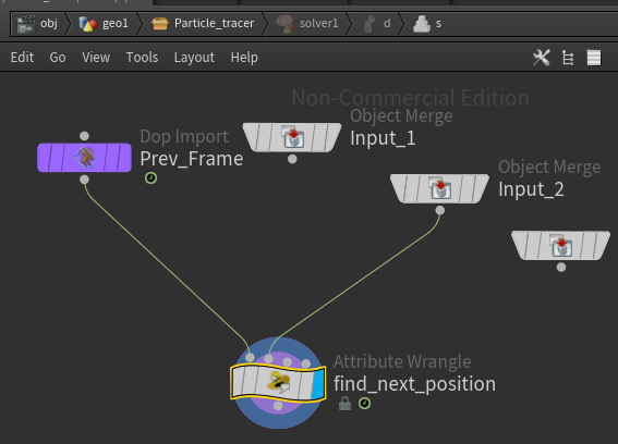
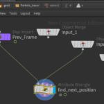
Finally its time to do the interesting part. Lay down a solver node and double click to enter inside the solver node. What makes solver special is that it gives us access to the geometry at the previous time step. Connect the Prev_Frame node with a new attribute wrangle node. Rename the new node to find next position, make sure to change the Run Over at primitives and connect the second input of particle tracer to the second input of the new wrangle node. The network should look similar to this:
Since the find next position node will do all the work, there is going to be a lot of code here.
First we are going to create a slider that will help us choose the number of points to be taken into account during velocity interpolation and a slider to define at what distance the points will be considered. Here we also define a scale velocity slider that will be used at a later time. The if statement ensures that even if one uses wrong number of interpolation nodes the code will still work. however the interpolation method will be similar to nearest neighbor interpolation.
|
|
int Nint = chi('N_points_velocity_interpolation'); float search_radius = ch('Search_radius'); float scale_vel = ch('Velocity_scale'); if (Nint <= 0) Nint = 1; |
Next step is to find how many vertices the primitive has.
|
|
int Nverts = primvertexcount(0, @primnum); |
There should be at least one vertex and the following lines get the point index and the position of that last vertex in the primitive
|
|
int pt_last = primpoint(0, @primnum, Nverts-1); vector pos_last = point(0,'P', pt_last); |
Now we can search for
Nint nearest points within a sphere with radius
search_radius
|
|
int closept[] = pcfind(1, "P", @P, search_radius, Nint); |
The array
closept contains the ids of the velocity points that satisfy the above criteria. After we initialize some help variables we loop through the velocity points. (Note that the code will use Inverse Distance Weighting Interpolation IDW)
For each velocity point get the velocity vector and calculate the distance of the current trajectory point with the velocity interpolation point.
|
|
float w[]; float sum_w = 0; vector vel[]; foreach (int pt; closept){ int out; vector interp_vel = pointattrib(1, 'v', pt, out); float d = distance(pos_last, point(1, 'P', pt)); |
According to IDW if the distance is 0 set directly the velocity equal to the velocity node. When this condition is true the code removes any other weight and velocity, appends only the values of this velocity node and exits the loop.
|
|
if (d == 0){ resize(w, 0); resize(vel, 0); sum_w = 1; append(vel, interp_vel); append(w, 1); break; |
if the distance is not zero, the weight of this velocity point is set equal to the inverse distance
|
|
else{ append(w, 1/d); sum_w += 1/d; append(vel, interp_vel); } |
Now we can calculate the velocity of the point
|
|
vector my_vel = {0,0,0}; for (int i = 0; i < len(w); ++i){ my_vel.x = w[i]*vel[i].x; my_vel.y = w[i]*vel[i].y; my_vel.z = w[i]*vel[i].z; } my_vel = my_vel/sum_w; |
Finally we can compute the position of the next point in the particle trajectory. Note that we multiply the calculated velocity with the scalar that has the effect of speeding up or slowing down the velocity.
|
|
vector new_pos = pos_last + my_vel*scale_vel; |
Although the following is not needed, will help us during visualization. The first line sets the calculated velocity as point attribute of the previous point and calculates the normal of the previous point so that it points in the new position.
|
|
setpointattrib(0, 'v', pt_last, my_vel, 'set'); vector normal_pt = new_pos - pos_last; setpointattrib(0, 'N', pt_last, normal_pt, 'set'); |
So far we have found the new position but we have to add it to the primitive.
|
|
int new_pt = addpoint(0, Nverts); setpointattrib(0, 'P', new_pt, new_pos, 'set'); addvertex(0, @primnum, new_pt); |
That concludes the code if this wrangle node. Here is the full code without interruptions
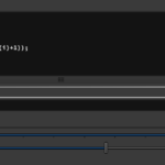
1 2 3 4 5 6 7 8 9 10 11 12 13 14 15 16 17 18 19 20 21 22 23 24 25 26 27 28 29 30 31 32 33 34 35 36 37 38 39 40 41 42 43 44 45 46 47 48 49 50 51 52 53 54 55 56 57 58 59 60 61 62 63 64 65 66 67 68 69 70 71 72 73 74 75 76 77 |
//Number of points involved in the velocity interpolation int Nint = chi('N_points_velocity_interpolation'); float search_radius = ch('Search_radius'); float scale_vel = ch('Velocity_scale'); if (Nint <= 0) Nint = 1; // find how many vertices exist in the primitive int Nverts = primvertexcount(0, @primnum); if (Nverts >= 1){ // get the id of the last one int pt_last = primpoint(0, @primnum, Nverts-1); //i@temp = pt_last; // position of last vertex vector pos_last = point(0,'P', pt_last); // Find the position of the last point in the primitive int closept[] = pcfind(1, "P", pos_last, search_radius, Nint); //i@Nfind = len(closept); // Calculate the distace from each velocity point float w[]; float sum_w = 0; vector vel[]; foreach (int pt; closept){ int out; // get the velocity of the pt point vector interp_vel = pointattrib(1, 'v', pt, out); // find the distance between the velocity point and the point in question float d = distance(pos_last, point(1, 'P', pt)); // If the distance is zero then assign this velocity // ignore the other values and exit the loop if (d == 0){ resize(w, 0); resize(vel, 0); sum_w = 1; append(vel, interp_vel); append(w, 1); break; } else{ append(w, 1/d); sum_w += 1/d; append(vel, interp_vel); } } // Next compute velocity as weighted average vector my_vel = {0,0,0}; for (int i = 0; i < len(w); ++i){ my_vel.x = w[i]*vel[i].x; my_vel.y = w[i]*vel[i].y; my_vel.z = w[i]*vel[i].z; } my_vel = my_vel/sum_w; // assign the velocity as attribute to the previous point setpointattrib(0, 'v', pt_last, my_vel, 'set'); // find the next position vector new_pos = pos_last + my_vel*scale_vel; // calculate the normal vector for the last position vector normal_pt = new_pos - pos_last; setpointattrib(0, 'N', pt_last, normal_pt, 'set'); // add the point in the primitive with id the next number int new_pt = addpoint(0, Nverts); setpointattrib(0, 'P', new_pt, new_pos, 'set'); addvertex(0, @primnum, new_pt); } |
Make sure that the blue flag is set to the wrangle node and exit the solver node. Pressing play will show the particle trajectories as lines.
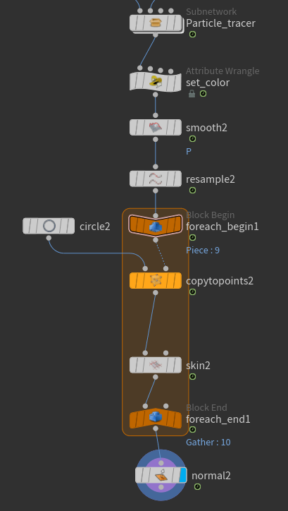
Particle trajectory appearance
The computation of particle tracking has finished in the previous section. Here we will work just on the appearance. First we will add color to the points according to velocity. To this end add another attribute wrangle node, rename it to set color and add the following lines. Press the button to generate the gui elements. This snippet calculates the velocity magnitude and assigns a color between green and red.
|
|
float min_vel = ch('Minimum_value'); float max_vel = ch('Maximum_value'); vector red = {0.9, 0, 0}; vector green = {0, 0.9, 0}; float l = length(@v); @Cd = lerp(green, red, fit(l, min_vel, max_vel, 0.0, 1.0)); |
Convert polylines to tubes
Depending on the velocity field the polyline may be jagged. Therefore we lay down 2 nodes. A smooth node and a resample node. Both of these nodes have their own parameters that define the smoothing amount resampling amount. Its best to play around with those values to find what looks better.
It is very common to display the particle trajectories as tubes. To achieve this in Houdini is trivial.
First create a cirlce node and scale it down to something that makes sense. In my example I set the Uniform Scale parameter to 0.004.
Now we are going to loop through the primitives (at the moment the number of primitives is equal to the initial number of particles). However we will do that using the For-Each Primitive node. This is going to lay down two nodes. A for each begin and a for each end. This is going to loop through the primitives and execute whatever nodes are in between. Add the copy to points and skin nodes as shown in the figure:
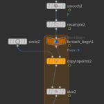
Last we add a normal node which corrects the face normals so that the polygon faces are lighted correctly