In spatial analysis it is very common to gather GIS layers from a variety of sources and more than often the layers may have different coordinate systems. Every GIS software know how to project each layer that comes with different projection information (The projection information is saved in a separate file with suffix *.prj) and can perform spatial analysis tasks on layers with different projection system.
In Matlab and R however the spatial analysis operations work only if the layers have the same coordinate system. Luckily both languages provide functions to convert between projections. Matlab introduced some functions that help with the transformation in the latest update 2020b. So the following will not work in any previous Matlab version not even in 2020a.
Matlab
First let’s bring a couple of data into Matlab workspace. The first layer is a point layer with well locations and the second layer contains the Subregions of the C2Vsim model groundwater basins. For the first layer the *.prj file is missing therefore the coordinate is unknown. For the second file we know from the report that the coordinate system is the EPSG:26910 – NAD83 / UTM zone 10N – Projected.
Mode info about EPSG see here
|
1 2 3 4 5 6 7 8 9 10 11 12 13 14 15 16 17 |
% For the well layer % Read the shapefile information wells_info = shapeinfo('CVwelldata'); % Read the shapefile geometry wells = shaperead('CVwelldata'); % For the Subregion layer % Read the shapefile information C2Vsim_basins_info = shapeinfo('C2Vsim_subBasins'); % Read the shapefile geometry C2Vsim_basins = shaperead('C2Vsim_subBasins'); |
The wells_info.CoordinateReferenceSystem returns an empty field because the projection information is missing. On the other hand C2Vsim_basins_info.CoordinateReferenceSystem returns the following structure
|
1 2 3 4 5 6 7 8 9 |
ans = projcrs with properties: Name: "NAD83 / UTM zone 10N" GeographicCRS: [1×1 geocrs] ProjectionMethod: "Transverse Mercator" LengthUnit: "meter" ProjectionParameters: [1×1 map.crs.ProjectionParameters] |
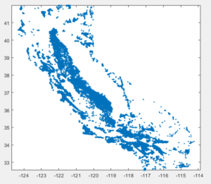
Unfortunately I’m not aware of any automated process to identify the projection system but we can make guesses by examining the coordinate values. If we plot the well data set we get the following image
|
1 2 |
plot([wells.X]', [wells.Y]','.') axis equal |
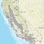
We can see that the range of X and Y coordinates is between -124 – -114 and 33 – 42. If you work with California data this range corresponds to the WGS 84 system with EPSG:4326. This is the coordinate system that many web applications use such as google maps, earth engine etc. use. We can easily verify our assumptions in matlab using the webmap tool. If the coordinate system is indeed 4326 then they should be projected in the right place.
|
1 2 3 |
webmap % starts the webmap wmmarker([wells.Y]', [wells.X]','Alpha',1, 'Color','green', 'IconScale', 0.2, ... 'Icon','http://maps.google.com/mapfiles/kml/shapes/shaded_dot.png'); |
We can see that the well locations fall in the right place. Now we can transform this to any coordinate system using. Note that you may have to switch X and Y
|
1 |
[Wx,Wy] = projfwd(projcrs(3310),[wells.Y]', [wells.X]'); |
Next we have to convert the basin coordinates from EPSG:26910 to EPSG:3310. I haven’t found yet and way to do this transformation using one line so I first convert from EPSG:26910 to EPSG:4326 using projinv and then convert to EPSG:3310. Also because the projinv and projfwd accept only X,Y coordinates not structures we have to loop through the polygons
|
1 2 3 4 |
for ii = 1:length(C2Vsim_basins) [lat,lon] = projinv(projcrs(26910),C2Vsim_basins(ii,1).X, C2Vsim_basins(ii,1).Y); [C2Vsim_basins(ii,1).X3310, C2Vsim_basins(ii,1).Y3310] = projfwd(projcrs(3310),lat, lon); end |
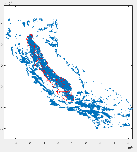
Now that the two layers have their coordinates on the same system we can overlay them

|
1 2 3 4 5 |
plot(Wx,Wy,'.') hold on for ii = 1:length(C2Vsim_basins) plot(C2Vsim_basins(ii,1).X3310, C2Vsim_basins(ii,1).Y3310,'r') end |
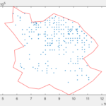
Now that the data sets share the same coordinate system we can do spatial operations. For example we can isolate the wells that are located in the southern most sub-basin of the Central Valley.
 |
|
R
In R the spatial transformations are even easier. First load the library library("rgdal")
The transformation between coordinate system is just one line of code
|
1 2 3 4 5 6 7 8 9 10 11 |
# Read the data sets wells <- readOGR(dsn = '.', layer = 'CVwelldata') C2Vsim_basins <- readOGR(dsn = '.', layer = 'C2Vsim_subBasins') # Change the coordinate system to 3310 C2Vsim_basins_3310 <- spTransform(C2Vsim_basins, CRS("+init=epsg:3310")) # Because the wells have no coordinate information first we have to assign the correct one # we know that this is the 4326 crs(wells) <- CRS('+init=EPSG:4326') # Now we can make the transformation wells_3310 <- spTransform(wells, CRS("+init=epsg:3310")) |

