Lets suppose that two shapes describe the same geographic area each digitized by different people at different coordinate system e.g. different transform, rotation and scaling and you want to match the two shapes.

This may seem unusual task. Unfortunately I had to deal with it. In particular I was given a Modflow model which was rotated and translated so that the left bottom corner of the domain was the (0,0) coordinate and I had to convert it to the coordinate system I was using. Also the two models described the same area, yet the digitization of the outline was made by different people therefore there were significantly different in the details.

The approach I took might not be the best and I welcome suggestions.

As I have some background in optimization I decided to run an optimization problem where the decision variables would be the translate, rotate and scale factors and the objective function would be the minimization of the area that remains after a Boolean subtraction between the two shapes.

Although this may sound a bit complicated task, it turned out to be relatively trivial using Matlab as it provides all the functionality one may need.

Lets name the outline of the modflow domain, modflow shape and the one with actual coordinates the target shape.

First we need to have the two shapes into Matlab workspace. For the modflow shape I rasterized the modflow grid and convert it to polygon shapefile in QGIS. The target shape was already a shapefile. The two shape files can be easily loaded with the shaperead matlab function:

 

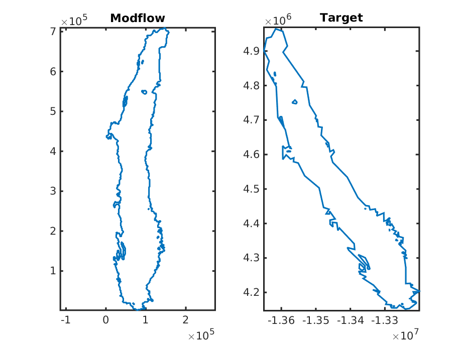
It is quite important to have the two shapefiles somehow simplified otherwise the boolean operations might slow down the process.

Next we have to write the objective function. The arguments will be a vector 4×1 (X, Y, R S) i.e. x,y translation, rotation and scaling.

Create a new file, e.g. obj_fun.m and paste the code from this link:

Now we are ready to run the optimization problem. I have found that the pattern search is very reliable optimization algorithm for this problem.

First I run the optimization without scaling because small changes can make big differences. This will give an idea about the scaling limits.

 

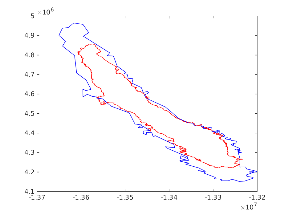
The figure above shows the result of the first optimization. The red shape is the translated and rotated geometry. The translation and rotation looks good. But definitely we need scaling to make it better. We can also estimate that the scaling factor has to be greater than 1 and less than 1.5. Therefore we will set those values as constrains. In addition we will set the starting point of the next optimization run the solution of the previous run.

The figure below shows the final results of the optimization run

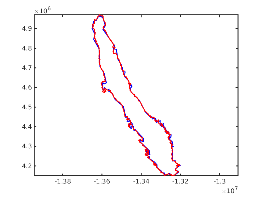
I should note that I had to perform quite a few optimization runs to reach this solution. In addition I performed few runs with fewer desicion variables. For example keep the rotation constant and optimize for scaling etc.

As you can see the result is not perfect and there are discrepancies especially in the north area. Therefore it may need to optimize for rotation.