The latest version of IWFM uses hdf output file format. This makes the reading output files a bit more difficult since the outputs are not in ASCII format but way more efficient. Luckily Matlab, R and many other languages can handle hdf formats quite easily.

Groundwater Zone Budget file

The first step to read any hdf file in matlab is to read the information that is contained in the file

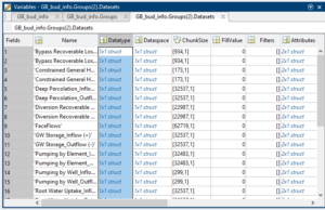
The GB_bud_info is a structure with many fields that contain plenty of useful information. After examining the structure in my version the GB_bud_info contained the field Groups, which has the following structure

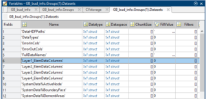
If we expand the dataset for the Layer1 we see the following structure

From this table we can find the row where each property is located . To read the data for a specific property we use the following. The Storage for example is the row 22. The following snippet loops through the layers and adds the entire storage from all layers

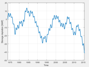
The units of the hdf file are in feet. Since this is storage the units are cubic feet. To generate the famous storage depletion plot of Central valley for example after we have calculated the above we can do the following

 

In the case of storage the data have dimensions as we see in the ChunkSize field 32537 and we can somewhat safely assume that the 1st row correspond to 1st element etc. However the ChunkSize for the Streams (rows 23,24) is 9885.

The size of the StreamBud  variable is 504×9885. Therefore from this matrix we cannot tell which element corresponds to the values. This information exists under Group(1).Datasets

The 6th row contains the correspondence between data and elements. To read it use

which returns a matrix 24×32537 (note that the above code transpose the output). Obviously the columns are related to the elements but how about the rows? This information exists in the 5th row of the above variable which we can read it as

The Colnames variable consist of 24 rows! The 3rd row is the Streams_Inflow (+). The elements that are associated with the stream budget are the nonzero ones in the 3rd row of the ids matrix which can be extracted easily

 

Extract Budget terms for a sub-region

In the following we are going to extract the groundwater pumping for the 21st subregion. Note that this is not a continuation of the above 

First we read the mesh information where the correspondence between subregions and mesh element is defined. For the following I’m using the latest version of the modeling which can be cloned from this repo. I also use one custom matlab function to read the element file which can be found in here

The pumping is not printed for all elements and not all layers pump from the same elements. The following is looping through the 4 layers of the models and extract which elements are associated with the budget terms. We also read the column names

In this version the column names consists of 26 rows and the rows 21-24 are related to pumping. However we are interested only in the negative terms which denote extraction from the groundwater. Besides the positive pumping is zero in the model. The rows 22 and 24 correspond to element and well pumping. 

Before assembling the budget terms we can find the elements of the subregion of interest. Here I’ll use the 21st subregion

The next snippet loops through the layers and extracts the element ids for the element and well pumping. If any element has no pumping then the id will be 0 so we remove the 0 entries. Last we read the data from the hdf5 file and sum the pumping from all the elements for each time step and save the results to a matrix.

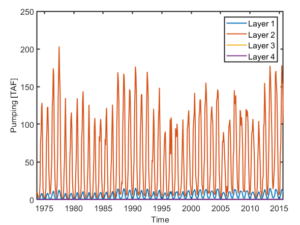
Now let’ s plot the pumping for each layer separately