3D Flow problem (hexahedral elements)

This example shows how to solve the groundwater flow equation using hexahedral elements. Here we choose quadratic elements however the procedure will be almost identical for linear elements. We also show how to deal with non-linear unconfined problems using a moving mesh approach. Finally we will show how to define general head boundary conditions and lateral flow boundaries.

Create 3D mesh
Hydraulic conductivity
Boundary conditions
Flux boundary conditions
Assemble
Unconfined solve

Create 3D mesh

The domain of the problem is given in a previous tutorial. In this example we will use the same mesh that was generated for the 2D flow problem. However we need to extrude the mesh in the z direction.

First we read the mesh from the Simple_quad.msh file.

[p_2d MSH_2d]=read_2D_Gmsh('Simple_quad');

Next we define the bottom and top elevation of the domain as inline functions of the x and y coordinates

top_func = @(x,y)30 - 0.01.*x + 0.04.*y;
bot_func = @(x,y)-20 - 0.02.*x - 0.01.*y;

and use the inline functions to compute the bottom and top elevations of the mesh nodes.

p_top = top_func(p_2d(:,1), p_2d(:,2));
p_bot = bot_func(p_2d(:,1), p_2d(:,2));

We can also plot them to make sure we have made the correct calculations

plot3(p_2d(:,1), p_2d(:,2), p_top, '.r')
hold on
plot3(p_2d(:,1), p_2d(:,2), p_bot, '.g')
view(60, 10)
grid on

To extrude the mesh in the z direction we need to define the number of layers and the distribution of layers. Here we will use a simple uniform distribution of 5 layers. For more advance options see the example of the Centerfor2points function.

A simple way to define uniform distribution in Matlab is to use the linspace function. The following line does two things. First the size of variable t determines the number of layers. The size is equal to 6 therefore after the extrude operation there will be 5 layers of 3D elements. The second thing is that it defines the distribution of the layers. For every mesh the elevations of the 6 layers will be scaled according to the distribution in t.

t = linspace(0,1,6);

Finally we extrude the mesh

[p MSH]=extrude_mesh(p_2d, MSH_2d, p_top, p_bot, t, 'quadratic');

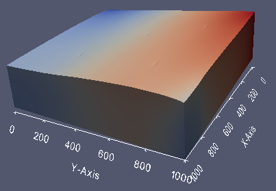
For quick review of the result we can plot the nodes just to make sure that we have the desired outcome. In matlab we cannot plot quadratic hexahedral elements so we plot just the nodes.

plot3(p(:,1), p(:,2), p(:,3),'.')
view(91,-6);

Hydraulic conductivity

In this example we will use an heterogenous hydraulic conductivity field which can be found in the DATA folder. The units of the field are m/day

load Kfield3D;

This is just a hypothetical example and we use a hypothetical grid that covers the domain

x_k=linspace(0,1000,size(Kfield,2));
y_k=linspace(0,1000,size(Kfield,1));
z_k=linspace(-51,80,size(Kfield,3));

and then we interpolate the hydraulic conductivity to mesh nodes

Kfield = Kfield/40;
Kx=interp3(x_k,y_k,z_k,Kfield,p(:,1),p(:,2),p(:,3));

and just for illustration lets define an anisotropic aquifer.

K = [Kx Kx/10 Kx/100];

Boundary conditions

Our example has two types of boundary conditions. General head boundary on the left, constant flux from the top and two lateral fluxes on the top right corner.

For the general head boundary conditions we will find the mesh node ids of the leftmost boundary which have zero x coordinate.

id = find(abs(p(:,1)<1));

We assing head value equal to the initial elevation and a relatively small value of 50 m^3/day for conductance.

GHB = [id top_func( p(id,1), p(id,2) ) 50*ones(length(id),1)];

Because we do not have any constant head boundary conditions we need to define an empty variable for that.

CH = [];

Flux boundary conditions

WELLS

For the flow conditions we make a distinction between those that are applied directly to nodes and those that are applied to elements.

Let's first deal we those applied to nodes which are somewhat easier to assign. Typical example are the wells. In our example we have 5 wells with coordinates

xw=[255 750 413 758 261];
yw=[802 738 514 293 192];

We also arbitarily set the top of the well screen to 10 m bellow the initial water table and the screen lenght equal to 30 m.

We define an empty variable that will hold the well rates.

FLUX_point = [];

The following loop does the folowing. For each well computes the distance between the well and the mesh nodes. However when we created the quadrilateral mesh we didnt force the mesh to use the wells as mesh nodes. Therefore we will assume that the wells correspond to the closest nodes. First we identify the minimum distance between each well and the mesh nodes and select all nodes that their distance is equal to the minimum. The number of selected nodes must be equal to the number of layers, in case of linear elements, or 2*Nlay - 1 in case of quadratic elements. In our case we defined 6 layers therefore for each well we should select 11 nodes.

Next we compute the elevation of the top and bottom of the well screen and identify which nodes are within the well screen and finally assign a well rate of 100 m^3/day for each well, i.e. we divide the well pumping rate by the number of mesh nodes that lay between the well screen.

for i = 1:length(xw)
    dst = sqrt((xw(i) - p(:,1)).^2 + (yw(i) - p(:,2)).^2);
    id = find(dst < min(dst)+0.1);
    z_top = p(id(1), 3) - 10;
    z_bot = z_top - 30;
    id_nd = find(p(id, 3) >= z_bot & p(id,3) <= z_top);
    FLUX_point = [FLUX_point; id(id_nd) -100/length(id_nd)*ones(length(id_nd),1)];
end

DIFFUSE RECHARGE

Next we define the diffuse recharge from the top of the aquifer To do so we need to a structure with several fields that will be described in the following paragraphs.

First we need to identify the id of the elements associated with the top recharge. By examining the 2D dimensional elements of the mesh which are given in the 3rd row of the MSH variable

MSH(3,1).elem
MSH(3,1).elem(1,1).type
MSH(3,1).elem(2,1).type

we see that there are 2 rows which contain elements of type quad. This is because we extruded a quadrilateral mesh to form a hexahedral mesh. If we extrude a 2D triangular mesh this structure will have two rows but one of them would be triangle type.

The second row of this structure contains the id of the top and bottom mesh which can be either quadrilateral or triangular and the first row contains the lateral boundaries, which are in any case quadrilaterals because the prism elements consist of two triangular faces on the top and bottom and 3 quadrilateral faces on the side.

The main conclusion from the above discussion is that the second row of the MSH(3,1).elem variable contains the elements of the top and bottop boundary and the second row the elements of the lateral boundaries. In addition the number of elements in MSH(3,1).elem(2,1).id should be always twice the number of elements of the 2D mesh MSH_2d(3,1).elem(1,1).id.

size(MSH(3,1).elem(2,1).id,1)

size(MSH_2d(3,1).elem(1,1).id,1)

Although we can identify the top or bottom elements by asking elements with z coordinates above or below a given value, there is a better way to to so by taking advantage the way the extrude function operates. In general the elements with node ids from 1 to size(p_2D,1) belong to the top layer

test = MSH(3,1).elem(2,1).id < size(p_2d,1);
id_top = find(sum(test ,2) == 9);

The above two lines first test which elements have ids with id number less than the size of the 2D mesh nodes. The elements that all of their vertices satisfy the above condition belong to the top layer. (Each element has 9 vetrices because the element of the top side of the domain is quadratic quadrilateral)

Now that we have identify the elements associated with diffuse recharge and we need to create a structure with the following fields:

The element ids

FLUX(1,1).id = id_top;

The recharge values for each element. Note that the order of the values should correspond to the order of ids when the recharge is heterogeneous

FLUX(1,1).val = 0.0008*ones(size(FLUX(1,1).id,1),1);

The dimension of the elements

FLUX(1,1).dim = 2;

The type of the elements

FLUX(1,1).el_type = 'quad';

The element order

FLUX(1,1).el_order = 'quadratic_9';

This is the row id in MSH(3,1).elem

FLUX(1,1).id_el = 2;

LATERAL FLUXES

For the lateral boundaries we will do exactly as above yet we will add one more option. The first lateral flow boundary is described by the plane with x and y coordinates along the line (800, 1000) -- (1000, 1000) and any z. To identify the elements that satisfy this condition we will loop through the corner element nodes and test whether they satisfy this condition

clear test
for k=1:4
    test(:, k)=(p(MSH(3, 1).elem(1, 1).id(:, k), 1) > 799 & p(MSH(3, 1).elem(1, 1).id(:, k), 2) > 999);
end

The elements that have all 4 corners satisfing the condition are associated with this flux boundary condition. Note that if the 4 corner nodes of the element satisfy the above condition then all the remaining 5 nodes will do as well.

FLUX(2,1).id = find(sum(test, 2) == 4);
FLUX(2,1).val = -1e-2*ones(size(FLUX(2, 1).id, 1), 1); % we assign an arbitary value here
FLUX(2,1).dim = 2;
FLUX(2,1).el_type = 'quad';
FLUX(2,1).el_order = 'quadratic_9';
FLUX(2,1).id_el = 1;

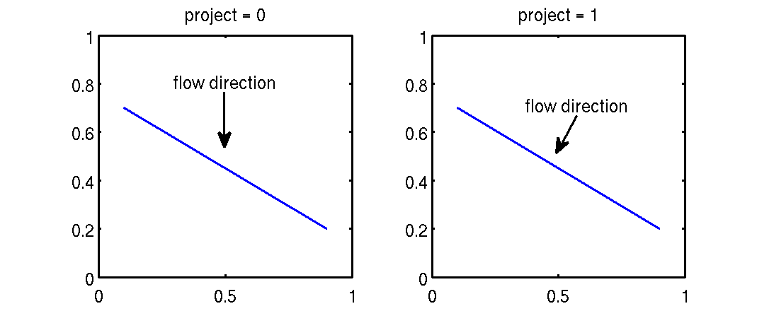
The next field is a new one. It simply states that the value in FLUX(2,1).val is applied over the actual area of the element regardless its orientation.

FLUX(2,1).project = 1;

The following plot explains graphically the difference between to two options. When project is equal to zero we assume that the direction of flow is vertical. When project is set equal to 1 then the flow direction is normal to the element face. Ommiting the project field does not generate an error but it will get 0 value by default.

For the second lateral flow boundary we will do exactly the same using a different condition

clear test
for k=1:4
    test(:, k)=(p(MSH(3, 1).elem(1, 1).id(:, k), 1) > 999 & p(MSH(3, 1).elem(1, 1).id(:, k), 2) > 799);
end
FLUX(3,1).id = find(sum(test, 2) == 4);
FLUX(3,1).val = -1e-2*ones(size(FLUX(3, 1).id, 1), 1); % we assign an arbitary value here
FLUX(3,1).dim = 2;
FLUX(3,1).el_type = 'quad';
FLUX(3,1).el_order = 'quadratic_9';
FLUX(3,1).id_el = 1;
FLUX(3,1).project = 1;

Assemble

Now we are ready to assemble the RHS. Since we use GHB the actuall degrees of freedom is the number of descritization nodes plus the number of GHB nodes

N_tot = size(p, 1) + size(GHB, 1);
F= Assemble_RHS(N_tot, p, MSH, FLUX);
F_w = zeros(length(F),1);
F_w(FLUX_point(:,1), 1) = FLUX_point(:,2);

As the models get more and more complex it becomes very important to verify that we have selected the right nodes and elements to apply the boundary conditions conditions

plot3(p(:,1), p(:,2), p(:,3),'.')
hold on
id = F > 0;
plot3(p(id,1), p(id,2), p(id,3),'.r')
id = F < 0;
plot3(p(id,1), p(id,2), p(id,3),'.g')
view(130,32)
hold off

Last we assemble the LHS and solve

simopt.dim = 3;
simopt.el_type = 'hex';
simopt.el_order = 'quadratic_27';
simopt.int_ord = 3;
[Kglo H]= Assemble_LHS(p, MSH(4,1).elem(1,1).id, K, CH, GHB, simopt);
H=solve_system(Kglo,H,F+F_w);

Unconfined solve

The problem we are dealing here is actually non-linear because the aquifer is unconfined. Therefore we need to use an iterative solution scheme where every iteration the elevations of the top nodes are set equal to the hydraulic head. The iterative process is repeated until some error indicator becomes very small.

A very simple error indicator is the average discrepancy between the hydraylic head and the elevation of the top nodes

Np_per_lay  = size(p_2d,1);
err(1,1)=mean(abs(p(1:Np_per_lay,3)-H(1:Np_per_lay)));

The non-linear solution involves a while loop where the LHS and RHS are assembled using the modified mesh elevations.

This is just a iteration counter

iter = 2;
while 1

we update the mesh based on the new top elevation

    p_top=H(1:size(p,1)/(2*length(t)-1));
    [p MSH]=extrude_mesh(p_2d,MSH_2d,p_top,p_bot,t,'quadratic');

the flux structures will be identical in this example, however this is not always true

    F= Assemble_RHS(N_tot, p, MSH,FLUX);

We reassemble the conductance matrix and solve

    [Kglo H]= Assemble_LHS(p, MSH(4,1).elem(1,1).id, K, CH, GHB, simopt);
    H=solve_system(Kglo, H, F + F_w);

check for the converge of the non-linear problem

    err(iter,1)=mean(abs(p(1:Np_per_lay,3) - H(1:Np_per_lay)));

if the error is very small then stop.

    if err(iter, 1)  <0.01;break;end
    iter = iter + 1;

end
semilogy(err);
xlabel('Iteration #');
ylabel('Error')

Finally we will write the data to vtk format and visualize the solution using paraview

propND(1,1).name = 'head';
propND(1,1).val = H(1:size(p, 1));
propND(1,1).type = 'scalars';
WriteVtkMesh('hex_flow', MSH(4, 1).elem.id, p, propND, [], 'hex')