Flow simulation in 1D

This is a simple example on how to use the msim functions to solve the groundwater flow equations for 1D domains

Problem Description
Mesh Generation
Boundary Conditions - fluxes
Boundary Conditions - Constant head
Assemble the matrices
Solve

Problem Description

The domain a 10 km line. The left boundary is a specified constant head and the right side is a specified flux. In addition we assume uniform recharge. First we specify some generic simulation options into a struct variable

opt.dim = 1; %This is the dimension of the problem
opt.el_order = 'linear'; %This is the element order. The other option is 'quadratic'
opt.assemblemode = 'vect';%other options are 'nested' and 'serial'. However you should always use 'vect' or leave empty

Mesh Generation

Next we define the 1D mesh. The mesh generation for this problem is trivial and there is no need to use Gmsh

L = 10000; %m domain Length
% Discretize the domain into 5 m segments
p = [0:5:L]';
Np = size(p, 1); %Number of nodes

To Define the mesh we use a structure variable with 2 rows. The first row corresponds to the zero dimension elements (e.g. points) and the second row to 1D elements (lines). Each row has the field elem with 1 or more rows depending on the number of elements. Each row of elem has 2 fields. id and type. id are the ids f the elements and type is the type pf the elements. Here we have only one type of elements

MSH(1,1).elem(1,1).id = [1:Np]';
MSH(1,1).elem(1,1).type = 'point';
MSH(2,1).elem(1,1).id = [(1:Np-1)' (2:Np)'];
MSH(2,1).elem(1,1).type = 'line';

Boundary Conditions - fluxes

The fluxes are divided into two categories. Those that are applied on elements and those that are applied on nodes. To account for the element fluxes we define the following structure:

FLUX(1,1).id = (1:length(MSH(2,1).elem(1,1).id))';
FLUX(1,1).val = 2e-5 * ones(length(FLUX(1,1).id), 1);
FLUX(1,1).dim = 1;% This is the dimension of the elements
FLUX(1,1).el_type = 'line'; %ths is unnecessary for 1D problems
FLUX(1,1).el_order = 'linear';
FLUX(1,1).id_el = 1; %This is the index in the Mesh.elem field
FLUX(1,1).assemblemode = 'vect';

Next we will defined 2 point sources which extract water from the domain (e.g. wells). Let's assume that the sources are are located at x = 403 and 825 m. However, since the mesh has been created before the definition of the point sources we will assing the fluxes to the nearets node.

[~, id1] = min(abs(403 - p));
[~, id2] = min(abs(825 - p));
FLUX_point = [[id1;id2] [-0.05; -0.05]];

Last we will assign the flux boundary at the right side of the domain

FLUX_point = [FLUX_point; Np -0.01];

Boundary Conditions - Constant head

This is a simple matrix where the first column is the id of the node and the second column is the specified value

CH = [1 30];

Assemble the matrices

Before assembling the matrices we need to define a hydraulic conductivity. We will define the hydraulic conductivity as random variable.

K = normrnd(50, 10, 100, 1);
x = linspace(0, L, 100)';
Knd = interp1q(x, K, p);
Tnd = Knd *1;

Assemble the left hand side matrix

[Kglo, H] = Assemble_LHS(p, MSH(2,1).elem(1,1).id, Tnd, CH, [], opt);

Assemble the right hand side matrix

F_rch= Assemble_RHS(length(H), p, MSH, FLUX);

The Assemble RHS function essentially distributes the element fluxes to the mesh nodes. Now we have to add the point fluxes to the output of the RHS assemble

F_rch(FLUX_point(:, 1), 1) = F_rch(FLUX_point(:, 1), 1) + FLUX_point(:, 2);

Solve

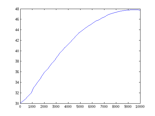
Now we can solve the problem by invoking the following function and plot the results

Head = solve_system(Kglo, H, F_rch);
plot(p, Head)