At large scales, rivers are delineated as lines. Typically river network data are in the form of polyline shapefile. To convert polyline network to polygon nework that is consistent is a quite challenging task. In GIS, the buffer approach is not returning the desired results as it returns a rounded buffer around the end polyline points.
For example, using the fixed distance buffer in QGIS with one segment the result is the following:
where each polyline segment creates a buffer polygon that overlaps with other.
The proposed workflow is not ideal but tackles some of the issues, while it returns a continuous representation of the river using polygons.
However the method is quite involved as requires some Matlab coding, and some experience with Houdini. A great advantage of the workflow is that it is non destructive, which means that modifications of the original input shapefile propagated at the end result without additional work.
Starting with Matlab, first we read the polyline shapefile:
|
|
cvhm_stream = shaperead('gis_data/CVHM_streams'); |
Each river consists of multiple polyline segments. Therefore we have to group them. Here we use the field NAME to group the rivers.
1 2 3 4 5 6 7 8 9 10 11 12 13 14 15 16 17 18 19 20 21 22 23 24 25 26 27 28 29 30 31 |
CVHMSTRM(1,1).Name = cvhm_stream(1,1).NAME; CVHMSTRM(1,1).segments(1,1).X = cvhm_stream(1,1).X; CVHMSTRM(1,1).segments(1,1).Y = cvhm_stream(1,1).Y; CVHMSTRM(1,1).segments(1,1).CELLNUM = cvhm_stream(1,1).CELLNUM; CVHMSTRM(1,1).segments(1,1).row = cvhm_stream(1,1).ROW; CVHMSTRM(1,1).segments(1,1).col = cvhm_stream(1,1).COLUMN_; for ii = 2:size(cvhm_stream,1) new_river = true; for jj = 1:size(CVHMSTRM,1) if strcmp(CVHMSTRM(jj,1).Name, cvhm_stream(ii,1).NAME) % add a segment to an existing river Nseg = size(CVHMSTRM(jj,1).segments,1); CVHMSTRM(jj,1).segments(Nseg+1,1).X = cvhm_stream(ii,1).X; CVHMSTRM(jj,1).segments(Nseg+1,1).Y = cvhm_stream(ii,1).Y; CVHMSTRM(jj,1).segments(Nseg+1,1).CELLNUM = cvhm_stream(ii,1).CELLNUM; CVHMSTRM(jj,1).segments(Nseg+1,1).row = cvhm_stream(ii,1).ROW; CVHMSTRM(jj,1).segments(Nseg+1,1).col = cvhm_stream(ii,1).COLUMN_; new_river = false; break; end end if new_river Nriv = size(CVHMSTRM,1); CVHMSTRM(Nriv+1,1).Name = cvhm_stream(ii,1).NAME; CVHMSTRM(Nriv+1,1).segments(1,1).X = cvhm_stream(ii,1).X; CVHMSTRM(Nriv+1,1).segments(1,1).Y = cvhm_stream(ii,1).Y; CVHMSTRM(Nriv+1,1).segments(1,1).CELLNUM = cvhm_stream(ii,1).CELLNUM; CVHMSTRM(Nriv+1,1).segments(1,1).row = cvhm_stream(ii,1).ROW; CVHMSTRM(Nriv+1,1).segments(1,1).col = cvhm_stream(ii,1).COLUMN_; end end |
The grouped rivers are stored into a temporary CVHMSTRM variable. Each polyline segment has shared nodes with other polyline segments, which are supposed to be connected. Here we make a unique list of river nodes.
1 2 3 4 5 6 7 8 9 10 11 12 13 14 15 16 17 18 19 20 |
for ii = 1:size(CVHMSTRM,1) CVHMSTRM(ii,1).ND = []; for jj = 1:size(CVHMSTRM(ii,1).segments,1) [Xs, Ys] = polysplit(CVHMSTRM(ii,1).segments(jj,1).X, CVHMSTRM(ii,1).segments(jj,1).Y); for kk = 1:size(Xs,1) for mm = 1:length(Xs{kk,1}) if isempty(CVHMSTRM(ii,1).ND) CVHMSTRM(ii,1).ND = [Xs{kk,1}(mm) Ys{kk,1}(mm)]; else dst = sqrt((CVHMSTRM(ii,1).ND(:,1) - Xs{kk,1}(mm)).^2 + ... (CVHMSTRM(ii,1).ND(:,2) - Ys{kk,1}(mm)).^2); if min(dst) > 0.1 CVHMSTRM(ii,1).ND = [CVHMSTRM(ii,1).ND;... Xs{kk,1}(mm) Ys{kk,1}(mm)]; end end end end end end |
Now that we have a list of unique river nodes we can create a graph, which is a structure that identifies the connections between nodes.
1 2 3 4 5 6 7 8 9 10 11 12 13 14 15 16 17 18 19 20 |
for ii = 1:size(CVHMSTRM,1) CVHMSTRM(ii,1).G = graph; for jj = 1:size(CVHMSTRM(ii,1).segments,1) [Xs, Ys] = polysplit(CVHMSTRM(ii,1).segments(jj,1).X, CVHMSTRM(ii,1).segments(jj,1).Y); for kk = 1:size(Xs,1) for mm = 1:length(Xs{kk,1})-1 dst = sqrt((CVHMSTRM(ii,1).ND(:,1) - Xs{kk,1}(mm)).^2 + ... (CVHMSTRM(ii,1).ND(:,2) - Ys{kk,1}(mm)).^2); id1 = find(dst < 0.1); dst = sqrt((CVHMSTRM(ii,1).ND(:,1) - Xs{kk,1}(mm+1)).^2 + ... (CVHMSTRM(ii,1).ND(:,2) - Ys{kk,1}(mm+1)).^2); id2 = find(dst < 0.1); if id1 ~= id2 Newedge = table([id1 id2], jj, 'VariableNames',{'EndNodes','seg_id'}); CVHMSTRM(ii,1).G = addedge(CVHMSTRM(ii,1).G, Newedge); end end end end end |
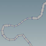
Graphs are powerful data classes that provide many functionalities. An example is the ability to plot them.
|
|
ii = 8; p = CVHMSTRM(ii,1).G.plot; p.XData = CVHMSTRM(ii,1).ND(:,1); p.YData = CVHMSTRM(ii,1).ND(:,2); p.NodeLabel = [1:size(CVHMSTRM(ii,1).ND,1)]; |
With the river graphs at our disposal we are able to identify the main rivers and separate them from the tributaries. The following lengthy code does two things. First Identifies the longest paths which are supposed to be the main rivers and the remaining paths connected to the longest one. Secondly calculates normal vectors for each river node. For the nodes that are connected to only one segment, the normal is equal to the segment normal. For the nodes that are connected to two segments the normal is the average of the two segment normals. Normals will be used later to create the river polygons.
1 2 3 4 5 6 7 8 9 10 11 12 13 14 15 16 17 18 19 20 21 22 23 24 25 26 27 28 29 30 31 32 33 34 35 36 37 38 39 40 41 42 43 44 45 46 47 48 49 50 51 52 53 54 55 56 57 58 59 60 61 62 63 64 65 66 67 68 69 70 71 72 73 74 75 76 77 |
for ii = 1:size(CVHMSTRM,1) clear PTHS NRM % find the terminal nodes id_term = find(CVHMSTRM(ii,1).G.degree == 1); if length(id_term) == 2 % there is only one path PTHS{1,1} = shortestpath(CVHMSTRM(ii,1).G, id_term(1), id_term(2)); else nds = []; for m = 1:length(id_term) for n = m+1:length(id_term) if m ~= n nds = [nds; id_term(m) id_term(n) length(shortestpath(CVHMSTRM(ii,1).G, id_term(m), id_term(n)))]; end end end [cc, dd] = sort(nds(:,3),'descend'); PTHS{1,1} = shortestpath(CVHMSTRM(ii,1).G, nds(dd(1),1), nds(dd(1),2)); nd_started_from = [nds(dd(1),1); nds(dd(1),2)]; for m = 2:length(dd) tmp1 = nds(dd(m),1); tmp2 = nds(dd(m),2); if isempty(find(nd_started_from == tmp1, 1)) PTHS{m,1} = shortestpath(CVHMSTRM(ii,1).G, tmp1, tmp2); nd_started_from = [nd_started_from; tmp1]; else if isempty(find(nd_started_from == tmp2, 1)) PTHS{m,1} = shortestpath(CVHMSTRM(ii,1).G, tmp2, tmp1); nd_started_from = [nd_started_from; tmp2]; end end end end for jj = 1:size(PTHS,1) for k = 1:length(PTHS{jj,1}) if k == 1 a = [CVHMSTRM(ii,1).ND(PTHS{jj,1}(k),:) 0]; b = [CVHMSTRM(ii,1).ND(PTHS{jj,1}(k+1),:) 0]; dm = b; dm(3) = pdist([a;b]); aver = false; elseif k == length(PTHS{jj,1}) a = [CVHMSTRM(ii,1).ND(PTHS{jj,1}(k-1),:) 0]; b = [CVHMSTRM(ii,1).ND(PTHS{jj,1}(k),:) 0]; dm = b; dm(3) = pdist([a;b]); aver = false; else a = [CVHMSTRM(ii,1).ND(PTHS{jj,1}(k-1),:) 0]; b = [CVHMSTRM(ii,1).ND(PTHS{jj,1}(k),:) 0]; c = [CVHMSTRM(ii,1).ND(PTHS{jj,1}(k+1),:) 0]; aver = true; end if jj > 1 && CVHMSTRM(ii,1).G.degree(PTHS{jj,1}(k)) == 3 aver = false; end if aver dm = b; dm(3) = pdist([a;b]); crs = cross(b-a,dm-a); N1 = crs/sqrt(sum(crs.^2)); dm = c; dm(3) = pdist([b;c]); crs = cross(c-b,dm-b); N2 = crs/sqrt(sum(crs.^2)); N = (N1+N2)/2; else crs = cross(b-a,dm-a); N = crs/sqrt(sum(crs.^2)); end NRM{jj,1}(k,:) = N; if jj > 1 && CVHMSTRM(ii,1).G.degree(PTHS{jj,1}(k)) == 3 PTHS{jj,1}(k+1:end) = []; break; end end end CVHMSTRM(ii,1).PATHS = PTHS; CVHMSTRM(ii,1).NORMS = NRM; end |
Finally for each river a width and flow rate is added. While the width is a required information for the method the flow rate could be omitted. However when I export the river polygons I would like to have the flow rate associated with each polygon. The code to add width depends on the application and is not shown here.
Last we write the river information into files for reading into Houdini. Note that the coordinate values are divided by a large constant 100000. This is because software like Houdini, blender etc do not handle very well large coordinate values.
|
|
cnt = 1; for ii = 1:size(CVHMSTRM,1) for mm = 1:size(CVHMSTRM(ii,1).PATHS,1) fid = fopen(['temp_stream' num2str(cnt) '.txt'], 'w'); fprintf(fid, '%d\n', length(CVHMSTRM(ii,1).PATHS{mm, 1})); fprintf(fid, '%f %f %f %f %f %f %f %f\n',... [CVHMSTRM(ii,1).ND(CVHMSTRM(ii,1).PATHS{mm, 1}',:)/100000 zeros(length(CVHMSTRM(ii,1).PATHS{mm, 1}),1)... % P {x,y,z} CVHMSTRM(ii,1).NORMS{mm, 1}(:,1:2) zeros(length(CVHMSTRM(ii,1).PATHS{mm, 1}),1) ... % N{x,y,z} CVHMSTRM(ii,1).Path_nd_width{mm,1}' [CVHMSTRM(ii,1).Path_Flow{mm,1} 0]' ... ]'); fclose(fid); cnt = cnt + 1; end end |
The format of the files is very simple
|
|
Nnodes x y z nx ny nz width flow . . . |
Now its time to launch Houdini.
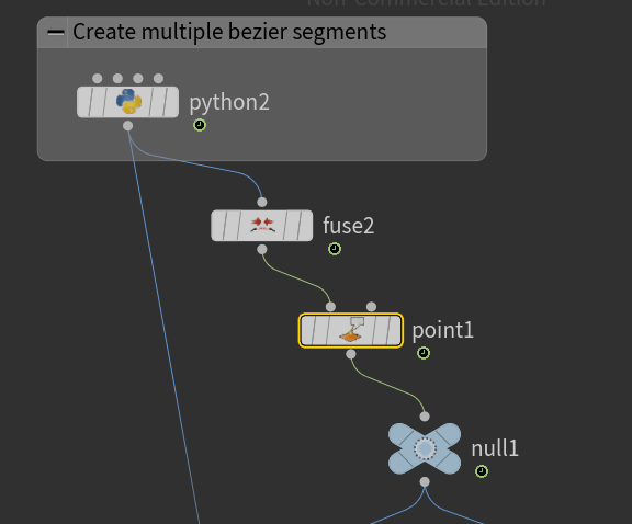
Place a python node inside a geometry node. (See this post on how to achieve this).
Add a new parameter to the python interface and make sure that the name of the parameter is
input_file . Then paste the following code to the python code area:
1 2 3 4 5 6 7 8 9 10 11 12 13 14 15 16 17 18 19 20 21 22 23 24 25 26 27 28 29 30 31 32 33 34 35 36 37 38 39 40 41 42 43 44 45 46 47 48 49 50 51 52 53 54 55 56 57 58 59 60 61 62 63 64 65 |
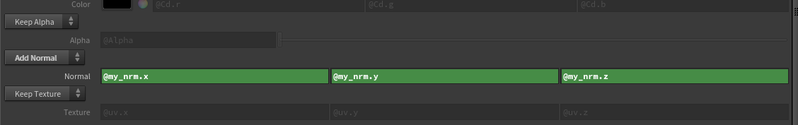
node = hou.pwd() geo = node.geometry() # Add code to modify contents of geo. # Use drop down menu to select examples. import csv import os def main(): geo = hou.pwd().geometry() geo.addAttrib(hou.attribType.Point, "my_nrm", hou.Vector3(0,0,0)) geo.addAttrib(hou.attribType.Point, "width", 0.0) geo.addAttrib(hou.attribType.Prim, "Qrate", 0.0) geo.addAttrib(hou.attribType.Global, "Nseg",0) inp_file = node.parm('input_file').eval() f = open(inp_file,'r') temp = f.readline() Nseg = int(temp)-1 geo.setGlobalAttribValue("Nseg", Nseg) pnt = {} nrm = {} w = {} q = {} for ii in range(0, Nseg+1): temp = f.readline() temp1 = temp.split(' ') pnt[ii] = hou.Vector3(float(temp1[0]), float(temp1[2]), float(temp1[1])) nrm[ii] = hou.Vector3(float(temp1[3]), float(temp1[5]), float(temp1[4])) w[ii] = float(temp1[6]) q[ii] = float(temp1[7]) for ii in range(0, Nseg): bz = geo.createBezierCurve(2, False, 2) bz.setAttribValue("Qrate", q[ii]) #temp = f.readline() #temp1 = temp.split(' ') readline = False ii = 0; for point in geo.iterPoints(): if readline: ii = ii +1 #temp = f.readline() #temp1 = temp.split(' ') point.setPosition(pnt[ii]) #point.setPosition(hou.Vector3(float(temp1[0]), float(temp1[2]), float(temp1[1]))) point.setAttribValue("my_nrm", nrm[ii]) point.setAttribValue("width", w[ii]) if readline: readline = False else: readline = True f.close() main() |
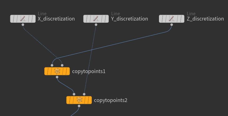
Next we are going to build a small graph to achieve the desired result.
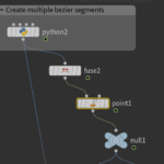
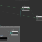
Right after python code we have to remove duplicated nodes using the Fuse node. Then we use the Point-Old node to set the normals:
I have also added a Null node that does nothing other than improving visibility and organizing the graph.
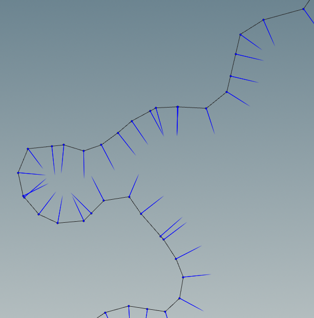
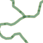
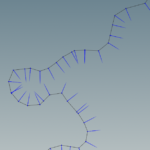
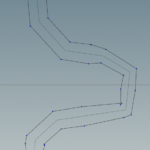
If we turn on the display points and display normals options we can see the river polyline, the points and the point normals.
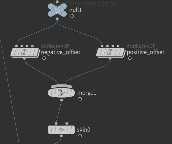
Next we lay down 2 Attribute VOP nodes. These nodes offset the main river by the width amount along the normal direction. In practice I created the positive offset and then duplicated to modify the negative offset.
By double clicking the attribute VOP (dive inside the node) we can modify the geometries at a different level. In addition we can see that the available nodes now are very different.
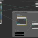
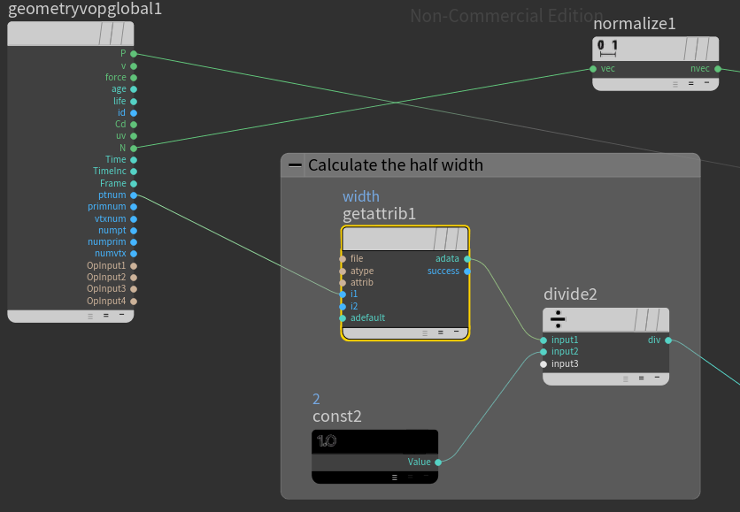
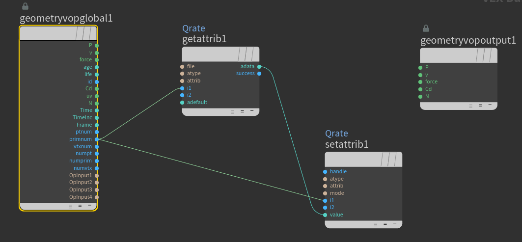
First we lay down a Get Attribute node to read the width information. For the Get Attribute to work we have to set float as Signature, First Input as Input method, Point as Attribute Class and type width for Attribute. As shown above the ptnum have to be connected to i1. In addition we lay down a constant float equal to 2 and a divide node to calculate the half width.
There is also a normalize node that is connected with the N value of the geometry. This is normalizing the normals of the nodes. The following figure shows the continuation of the Attribute VOP graph
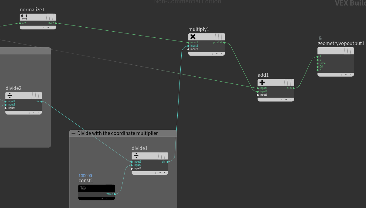
The outcome of half width is further divided by the same large constant we use when writing the houdini files, which is then multiplied by the point normalized normals and added to point Position values. Finally the result of add operation is connected to P geometry output node which shifts the nodes by half width amount. The negative offset node is identical with the exception that between the divide1 and multiply1 we have added a negate node.
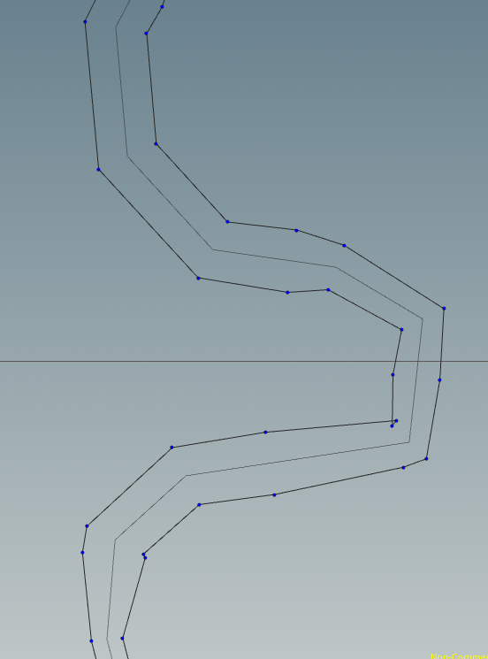
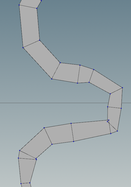
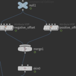
Next outside the Attribute VOP node we merge the two offset nodes and then add a skin node. The following figures show the result of the merge and the result of the skin node. For the skin to work properly we have to set some rules about which lines to connect. Set Quadrilaterals for connectivity. For Skin pick Skip every Nth primitive, and for N value use the expression
detail("../python2/","Nseg",0) which sets as N value the number of stream segments. Note that in the initial python code we set a global attribute Nseg.
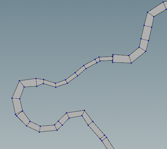
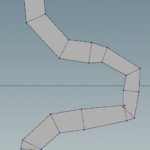
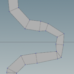
We can see in areas where the river has sharp bends some weird artifacts may be produced. These will be taken care later. However note how the river width changes smoothly between segments of different width.
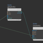
Somehow the Skin operator does not transfer the Qrate attribute to the polygons and sets all Qrates to 0. A simple attribute VOP takes care of that. A get and a set attribute node does exactly that.
Then the fuse node with a certain tolerance resolve the artifacts displayed above
Finally we use a python node to write the polygons into a file to export them into a suitable format using the following python code.
1 2 3 4 5 6 7 8 9 10 11 12 13 14 15 16 17 18 19 20 21 22 23 24 25 26 |
node = hou.pwd() geo = node.geometry() # Add code to modify contents of geo. # Use drop down menu to select examples. def main(): f = open("/home/giorgk/Documents/UCDAVIS/CVHM_NPSAT/temp_stream_out" + str(hou.intFrame()) + ".txt", 'w') f.write(str(len(geo.prims())) + "\n") for prim in geo.iterPrims(): q = prim.attribValue("Qrate") n = prim.numVertices() f.write(str(n) + " " + str(q) + "\n") coords = prim.vertices() for v in coords: X = v.point() XX = X.position() f.write(str(XX.x()) + " " + str(XX.z()) + "\n") #prim.setAttribValue("Qrate", float(n)) f.close() main() |